March 1, 2014
Science news cycle
From Piled Higher and Deeper. Substitute as necessary if your grandma is a scientist.
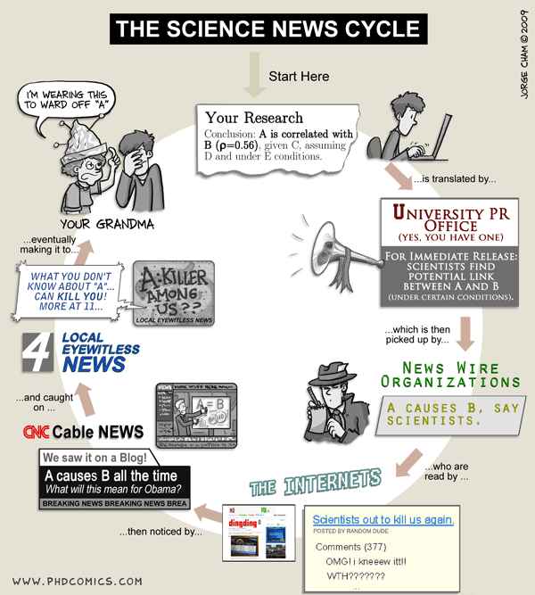
The only thing wrong with this is it gives too much credit to university PR departments.
From Piled Higher and Deeper. Substitute as necessary if your grandma is a scientist.
The only thing wrong with this is it gives too much credit to university PR departments.
The basic method is described on my Department home page. I have made some changes to the methodology this year, including shrinking the ratings between seasons.
Here are the team ratings prior to this week’s games, along with the ratings at the start of the seaso
| Current Rating | Rating at Season Start | Difference | |
|---|---|---|---|
| Roosters | 12.35 | 12.35 | 0.00 |
| Sea Eagles | 9.10 | 9.10 | 0.00 |
| Storm | 7.64 | 7.64 | 0.00 |
| Cowboys | 6.01 | 6.01 | -0.00 |
| Rabbitohs | 5.82 | 5.82 | 0.00 |
| Knights | 5.23 | 5.23 | 0.00 |
| Bulldogs | 2.46 | 2.46 | -0.00 |
| Sharks | 2.32 | 2.32 | -0.00 |
| Titans | 1.45 | 1.45 | -0.00 |
| Warriors | -0.72 | -0.72 | -0.00 |
| Panthers | -2.48 | -2.48 | 0.00 |
| Broncos | -4.69 | -4.69 | -0.00 |
| Dragons | -7.57 | -7.57 | 0.00 |
| Raiders | -8.99 | -8.99 | 0.00 |
| Wests Tigers | -11.26 | -11.26 | 0.00 |
| Eels | -18.45 | -18.45 | 0.00 |
Here are the predictions for Round 1. The prediction is my estimated expected points difference with a positive margin being a win to the home team, and a negative margin a win to the away team.
| Game | Date | Winner | Prediction | |
|---|---|---|---|---|
| 1 | Rabbitohs vs. Roosters | Mar 06 | Roosters | -2.00 |
| 2 | Bulldogs vs. Broncos | Mar 07 | Bulldogs | 11.70 |
| 3 | Panthers vs. Knights | Mar 08 | Knights | -3.20 |
| 4 | Sea Eagles vs. Storm | Mar 08 | Sea Eagles | 6.00 |
| 5 | Cowboys vs. Raiders | Mar 08 | Cowboys | 19.50 |
| 6 | Dragons vs. Wests Tigers | Mar 09 | Dragons | 8.20 |
| 7 | Eels vs. Warriors | Mar 09 | Warriors | -13.20 |
| 8 | Sharks vs. Titans | Mar 10 | Sharks | 5.40 |
As our regular readers will know, statschat bloggers go about educating the media in statistical literacy in various ways – making ourselves available to media, delivering workshops to working journalists and student journalists, and critiquing stats use in the media around us.
But we also have to look at the journalist pipeline – embedding statistical literacy in journalism students and their teachers. Over the last couple of years, Yours Truly, who spent many years of her life in newsrooms as a hack, latterly at the New Zealand Herald, has been banging that drum.
So it’s great news that the decision has been made to devise a unit standard in statistical thinking for the National Diploma in Applied Journalism that journalists follow on-the-job. This would be a Level 6 qualification and it would plug a gaping hole in the diploma. The unit standard doesn’t have a name yet (but I quite like the idea of something like “Demonstrate statistical literacy by ….”)
The reference group is below; we met this week to get things moving.
I’ll let you know from time to time how we’re going – and may well ask for your help in finding good case studies and Excel-based data sets to help journalists become familiar with statistical thinking and tools (Excel is a rarity in New Zealand newsrooms).
Just in from the Royal Statistical Society in the UK:
“Recent years have seen an encouraging amount of attention being paid to statistical accuracy in the media. This is not only because journalists can find meaty stories in catching a politician or organisation out with inaccurate figures. The increased amount of scrutiny in a changing media environment also means journalists themselves are under increasing pressure to get their facts and figures correct.
“The BBC has recognised this reality by creating a new post, Head of Statistics, with business reporter Anthony Reuben moving into the position after more than a decade at the corporation.”
Read more about this excellent piece of news on the Royal Statistical Society website here.
A new blog of science-themed links and (NZ) event listings, Science Club.
Their most recent post is for this story from the Guardian, which reports that one in every thirteen tweets contains swearing.
What do you think is the most commonly used swearword on Twitter? Well of course it is
There is, of course, substantial variation between users. Most of the people I follow are dragging the average down.
James Russell sent me a link to this story from a Canadian paper (originally from the Daily Telegraph). The Herald has it too, with a very slightly less naff picture. The research (open access) is good; the story is reasonably informative, but seriously credulous
Blood samples from over 17,000 generally healthy people were screened for 100 biomarkers, and those people monitored over five years.
In that time, 684 died from illnesses including cancer and cardiovascular disease. They all had similar levels of four biomarkers: albumin; alpha-1-acid glycoprotein; citrate, and a similar size of very-low-density lipoprotein particles.
Compare the last sentence to this graph from the research paper. The vertical axis is a combined score on the four biomarkers. The red dots are the people who died. As you can see, they didn’t all have similar values.
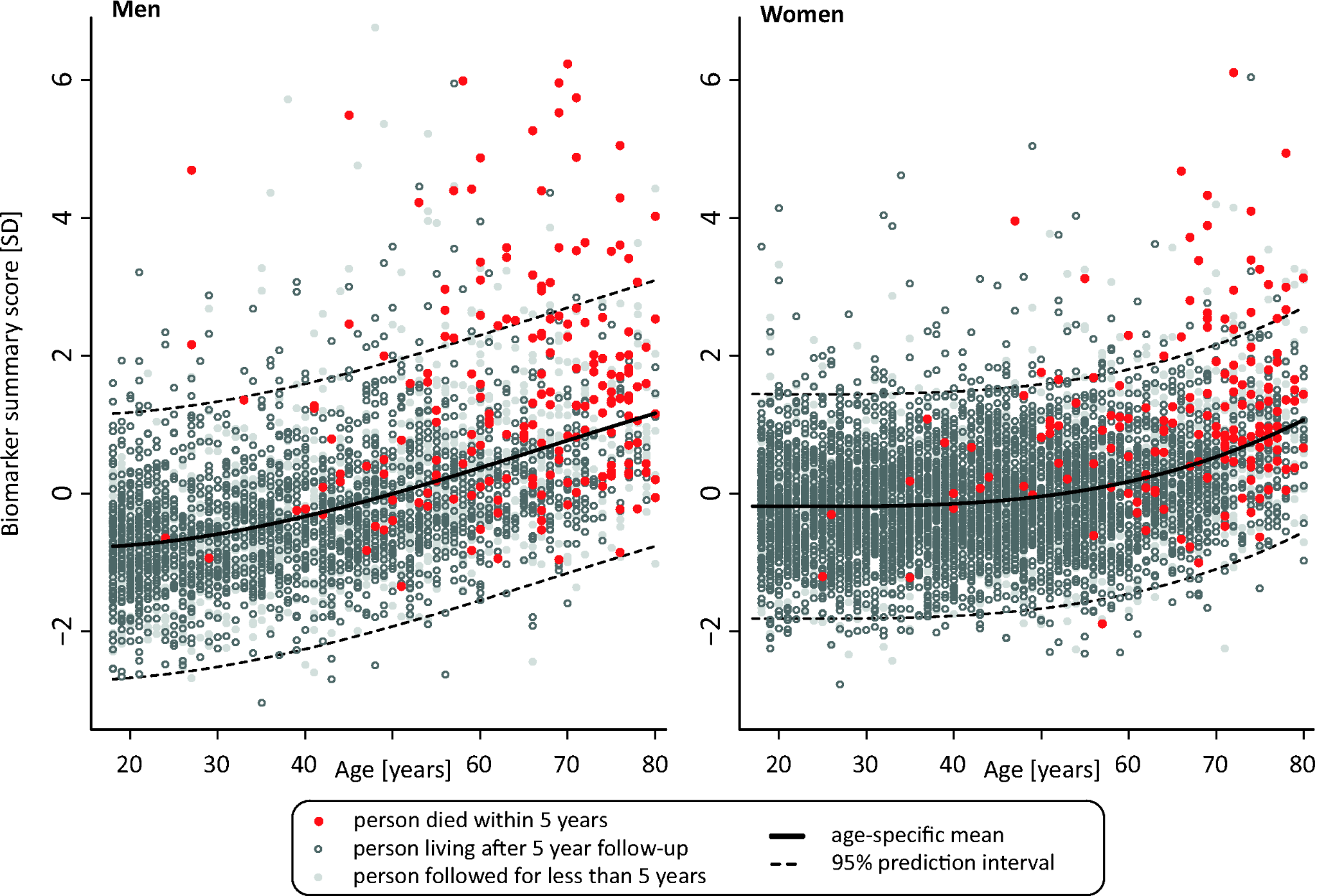
The research is impressive not because the prediction is very accurate, but because its less appalling inaccurate than usual. Using standard risk factors (age, sex, cholesterol, smoking, diabetes, cancer) if you picked a random person who died and one who didn’t die from their cohort there’s an 80% chance the one with the worse risk factors was the one who died. Adding the ‘death test’ measurements increases the probability to 83%. Asking an experienced nurse to guess would probably be more accurate (and cheaper), but is hard to automate.
Despite the impression from the headline and lead, if you’re asked to predict whether someone will live another year, based on this sort of information, the safe bet is “yes”. Even among the 1% of people with the very worst values of the ‘death test’ biomarkers, 80% lived for more than a year and half were still alive at the end of the five year study.
Interestingly, the two republished versions lack the last paragraphs of the original Telegraph story, which talk about whether the test is useful
“If the findings are replicated then this test is surely something we will see becoming widespread,” added Prof Perola.
“But at moment there is ethical question. Would someone want to know their risk of dying if there is nothing we can do about it?”
Dr Kettunen added: “Next we aim to study whether some kind of connecting factor between these biomarkers can be identified.
There’s a map going around Twitter, being described as the most popular band in each US state
Here’s the band that each state likes the most http://t.co/ANVw7ofA1s pic.twitter.com/HyI2u537rp
— Joseph Weisenthal (@TheStalwart) February 25, 2014
It’s a bit surprising that every state has a different favourite band, so I looked at the site listed on the map as the source. In fact, the listed bands are not the most popular ones in any of the states. They are something more interesting.
Paul Lamere used Spotify (and perhaps other social music-streaming services) to get music listening preferences for 200000 people. He then looked at which artist in the top 100 for a state had the worst ranking over the US as a whole. He forced the result to be different for every state by bumping the less-populous state to its next choice when there was a tie. So, as the title on the map actually says, these are the most distinctive bands for a state, not the most popular. They are caricatures, not photographs.
Since he had data based on postal code (ZIP code), it’s a pity he grouped these all the way up to the state level. It would have been interesting to see urban vs suburban vs rural differences, and the major geographical trends across states such as Texas.
From BBC News,in what’s actually a very good story, a picture of radiation from Fukushima spreading across the Pacific.
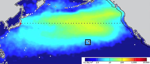
It’s actually a picture of a model prediction — the story is about using measurements of radiation from Fukushima to decide between two models that give predictions disagreeing by a factor of more than ten. That’s important not for the current plume, but in case there’s serious radiation release into the ocean from some reactor at some time in the future.
My point, though, is about colour scales. The yellow-green colour looks to be about halfway between reassuring non-irradiated dark blue and OMG WE’RE ALL GOING TO DIE!1!11!! dark red. It isn’t. The colour is on a logarithmic scale, so the maximum predicted concentration is about 30 becquerels per cubic metre, and the dark red is 10,000 becquerels per cubic metre. That sounds like a lot, but becquerels are very small — enough radioactive material to have one atom decaying per second. A banana contains about 15 becquerels of potassium-40.
In fact, the story says that 10,000 Bq/m3 , the dark red end of the scale, is the Canadian safety threshold for radiation in drinking water (ie, about 1.5 litres of water per banana of radiation), so the yellow colour on the map is about one third of one percent of the official safety threshold for drinking water.
There’s a good reason the graphic uses a log scale and a very low limit — on a scale that corresponded to risk the predicted Fukushima plume would be completely invisible. For scientific presentation, the graphic and its scaling are completely appropriate. For the top of a story on a mass-media website, perhaps not so much.
(via @zentree)
From Stuff the Herald
Rising economic confidence and “aggressive” marketing techniques are the driving factors behind an 8.9 million litre rise in alcohol availability last year, says one concerned health organisation.
That sounds like a lot, but the population is also increasing. So how does the alcohol per capita change? That might take some slight effort to work out, except that Statistics New Zealand puts it in the list of Key Facts for this data release and in the media release
The volume of pure alcohol available per person aged 15 years and over was unchanged, at 9.2 litres. This equates to an average of 2.0 standard drinks per person per day.
So, probably not due entirely to rising economic confidence and aggressive marketing techniques.
The basic method is described on my Department home page. I have made some changes to the methodology this year, including shrinking the ratings between seasons.
Here are the team ratings prior to this week’s games, along with the ratings at the start of the season.
| Current Rating | Rating at Season Start | Difference | |
|---|---|---|---|
| Crusaders | 7.89 | 8.80 | -0.90 |
| Sharks | 5.84 | 4.57 | 1.30 |
| Chiefs | 5.29 | 4.38 | 0.90 |
| Bulls | 3.55 | 4.87 | -1.30 |
| Brumbies | 3.15 | 4.12 | -1.00 |
| Stormers | 2.56 | 4.38 | -1.80 |
| Waratahs | 2.44 | 1.67 | 0.80 |
| Reds | 1.56 | 0.58 | 1.00 |
| Cheetahs | -0.02 | 0.12 | -0.10 |
| Hurricanes | -1.91 | -1.44 | -0.50 |
| Blues | -2.44 | -1.92 | -0.50 |
| Highlanders | -3.96 | -4.48 | 0.50 |
| Lions | -4.45 | -6.93 | 2.50 |
| Force | -6.14 | -5.37 | -0.80 |
| Rebels | -6.36 | -6.36 | -0.00 |
So far there have been 9 matches played, 3 of which were correctly predicted, a success rate of 33.3%.
Here are the predictions for last week’s games.
| Game | Date | Score | Prediction | Correct | |
|---|---|---|---|---|---|
| 1 | Crusaders vs. Chiefs | Feb 21 | 10 – 18 | 6.90 | FALSE |
| 2 | Cheetahs vs. Bulls | Feb 21 | 15 – 9 | -2.10 | FALSE |
| 3 | Highlanders vs. Blues | Feb 22 | 29 – 21 | -0.10 | FALSE |
| 4 | Brumbies vs. Reds | Feb 22 | 17 – 27 | 6.00 | FALSE |
| 5 | Sharks vs. Hurricanes | Feb 22 | 27 – 9 | 10.80 | TRUE |
| 6 | Lions vs. Stormers | Feb 22 | 34 – 10 | -8.10 | FALSE |
| 7 | Waratahs vs. Force | Feb 23 | 43 – 21 | 9.50 | TRUE |
Here are the predictions for Round 3. The prediction is my estimated expected points difference with a positive margin being a win to the home team, and a negative margin a win to the away team.
| Game | Date | Winner | Prediction | |
|---|---|---|---|---|
| 1 | Blues vs. Crusaders | Feb 28 | Crusaders | -7.80 |
| 2 | Rebels vs. Cheetahs | Feb 28 | Cheetahs | -2.30 |
| 3 | Stormers vs. Hurricanes | Feb 28 | Stormers | 8.50 |
| 4 | Chiefs vs. Highlanders | Mar 01 | Chiefs | 11.70 |
| 5 | Waratahs vs. Reds | Mar 01 | Waratahs | 3.40 |
| 6 | Force vs. Brumbies | Mar 01 | Brumbies | -6.80 |
| 7 | Bulls vs. Lions | Mar 01 | Bulls | 10.50 |
Recent comments