Stats Chat

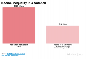
If you hadn’t seen this graph yet, you probably would have soon.

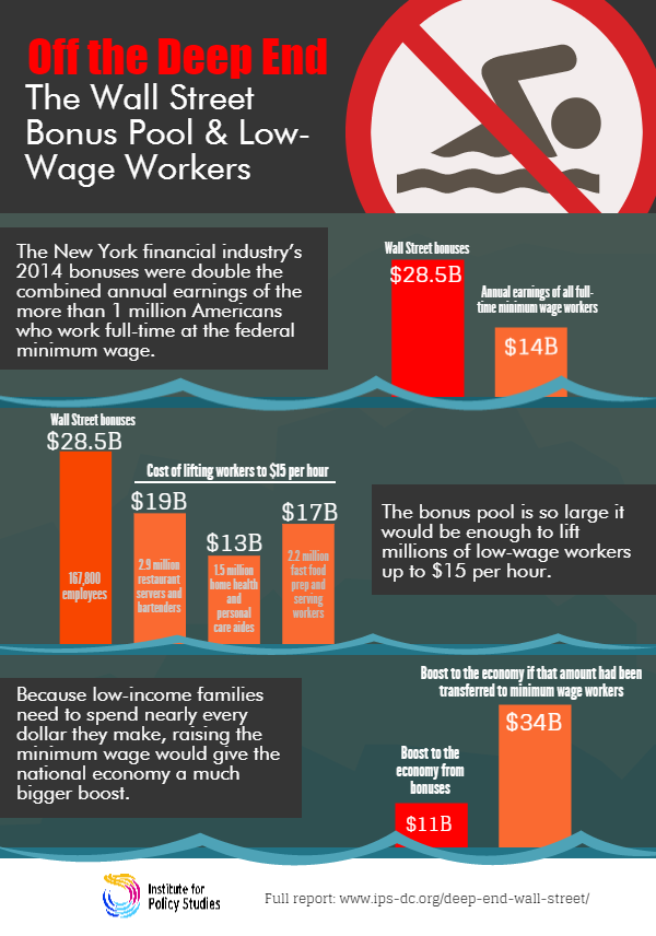
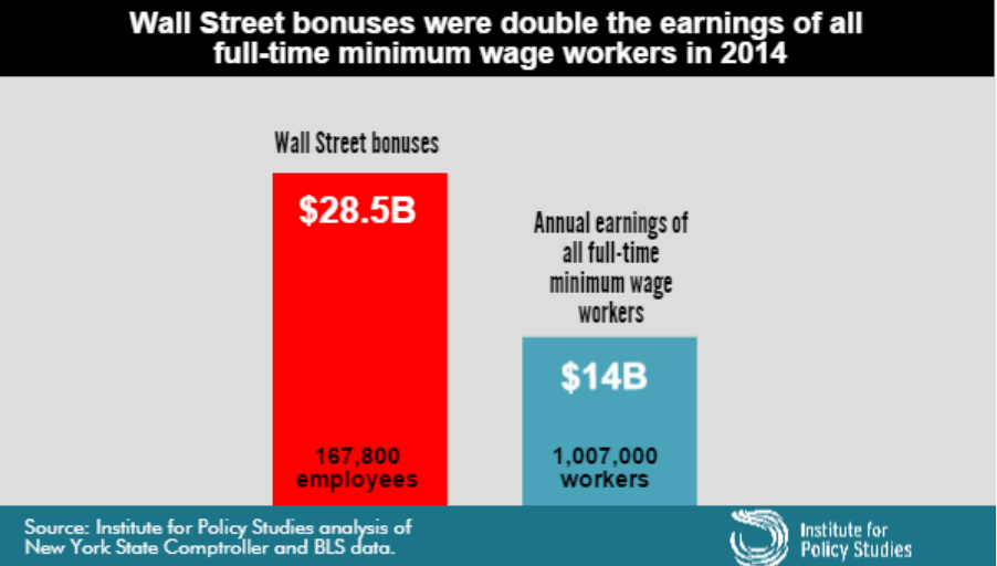
The claim “Wall Street bonus were double the earnings of all full-time minimum wage workers in 2014” was made by the Institute for Policy Studies (which is where I got the graph) and fact-checked by the Upshot blog at the New York Times, so you’d expect it to be true, or at least true-ish. It probably isn’t, because the claim being checked was missing an important word and is using an unfortunate definition of another word. One of the first hints of a problem is the number of minimum wage workers: about a million, or about 2/3 of one percent of the labour force.  Given the usual narrative about the US and minimum-wage jobs, you’d expect this fraction to be higher.

The missing word is “federal”. The Bureau of Labor Statistics reports data on people paid at or below the federal minimum wage of $7.25/hour, but 29 states have higher minimum wages so their minimum-wage workers aren’t counted in this analysis. In most of these states the minimum is still under $8/hr. As a result, the proportion of hourly workers earning no more than federal minimum wage ranges from 1.2% in Oregon to 7.2% in Tennessee (PDF).  The full report — and even the report infographic — say “federal minimum wage”, but the graph above doesn’t, and neither does the graph from Mother Jones magazine (it even omits the numbers of people)

On top of those getting state minimum wage we’re still short quite a lot of people, because “full-time” is defined by 35 or more hours per week at your principal job.  If you have multiple part-time jobs, even if you work 60 or 80 hours a week, you are counted as part-time and not included in the graph.

Matt Levine writes:

There are about 167,800 people getting the bonuses, and about 1.03 million getting full-time minimum wage, which means that ballpark Wall Street bonuses are 12 times minimum wage. If the average bonus is half of total comp, a ratio I just made up, then that means that “Wall Street” pays, on average, 24 times minimum wage, or like $174 an hour, pre-tax. This is obviously not very scientific but that number seems plausible.

That’s slightly less scientific than the graph, but as he says, is plausible. In fact, it’s not as bad as I would have guessed.

What’s particularly upsetting is that you don’t need to exaggerate or use sloppy figures on this topic. It’s not even that controversial. Lots of people, even technocratic pro-growth economists, will tell you the US minimum wage is too low.  Lots of people will argue that Wall St extracts more money from the economy than it provides in actual value, with much better arguments than this.

By now you might think to check carefully that the original bar chart is at least drawn correctly.  It’s not. The blue bar is more than half the height of the red bar, not less than half.

Thanks to Graeme Edgeler for winning our latest Stat of the Week competition and for his excellent explanation:

Statistic: “Māori adults have the highest levels of trust in the police, the health system & the courts. The lowest in the media”

Source: Tweet from Stats NZ

The statistic is written in a way that suggests Māori adults have the highest level of trust in the police etc., that is higher levels of trust than anyone else has in the police.

What the report actually shows is that the police etc. are the institutions in which Māori adults place the most trust as among institutions. It says nothing about whether Māori adults have more trust in them than anyone else. Anyone reading the tweet would think they did, but that was not even assessed.

It should be stat of the week, because, even if its not the most egregious stat this week, that fact that it is from Statistics New Zealand makes it worse.

Congratulations Graeme!

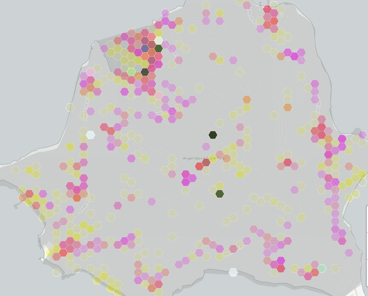
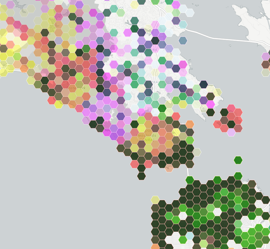
This is part of a social media map, of photographs taken in public places in the San Francisco Bay Area

The colours are trying to indicate three social media sites: Instagram is yellow, Flickr is magenta, Twitter is cyan.

Encoding three variables with colour this way doesn’t allow you to easily read off differences, but you can see clusters and then think about how to decode them into data. The dark green areas are saturated with photos.  Light green urban areas have Instagram and Twitter, but not much Flickr.  Pink and orange areas lack Twitter — mostly these track cellphone coverage and population density, but not entirely.  The pink area in the center of the map is spectacular landscape without many people; the orange blob on the right is the popular Angel Island park.

Zooming in on Angel Island shows something interesting: there are a few blobs with high density across all three social media systems. The two at the top are easily explained: the visitor centre and the only place on the island that sells food. The very dense blob in the middle of the island, and the slightly less dense one below it are a bit strange. They don’t seem to correspond to any plausible features.

My guess is that these are a phenomenon we’ve seen before, of locations being mapped to the center of some region if they can’t be specified precisely.

Automated data tends to be messy, and making serious use of it means finding out the ways it lies to you. Wayne Dobson doesn’t have your cellphone, and there isn’t a uniquely Twitter-worthy bush in the middle of Angel Island.

Each week, we would like to invite readers of Stats Chat to submit nominations for our Stat of the Week competition and be in with the chance to win an iTunes voucher.

Here’s how it works:

• Anyone may add a comment on this post to nominate their Stat of the Week candidate before midday Friday March 20 2015.
• Statistics can be bad, exemplary or fascinating.
• The statistic must be in the NZ media during the period of March 14 – 20 2015 inclusive.
• Quote the statistic, when and where it was published and tell us why it should be our Stat of the Week.

Next Monday at midday we’ll announce the winner of this week’s Stat of the Week competition, and start a new one.

(more…)

Some discussion on Twitter about political polling and whether political journalists understood the numbers led to the question:

If you poll 500 people, and candidate 1 is on 35% and candidate 2 is on 30%, what is the chance candidate 2 is really ahead?

That’s the wrong question. Well, no, actually it’s the right question, but it is underdetermined.

The difficulty is related to the ‘base-rate‘ problem in testing for rare diseases: it’s easy to work out the probability of the data given the way the world is, but you want the probability the world is a certain way given the data. These aren’t the same.

If you want to know how much variability there is in a poll, the usual ‘maximum margin of error’ is helpful.  In theory, over a fairly wide range of true support, one poll in 20 will be off by more than this, half being too high and half being too low. In theory it’s 3% for 1000 people, 4.5% for 500. For minor parties, I’ve got a table here. In practice, the variability in NZ polls is larger than in theoretically perfect polls, but we’ll ignore that here.

If you want to know about change between two polls, the margin of error is about 1.4 times higher. If you want to know about difference between two candidates, the computations are trickier. When you can ignore other candidates and undecided voters, the margin of error is about twice the standard value, because a vote added to one side must be taken away from the other side, and so counts twice.

When you can’t ignore other candidates, the question isn’t exactly answerable without more information, but Jonathan Marshall has a nice app with results for one set of assumptions. Approximately, instead of the margin of error for the difference being (2*square root (1/N)) as in the simple case, you replace the 1 by the sum of the two candidate estimates, so  (2*square root (0.35+0.30)/N).  The margin of error is about 7%.  If the support for the two candidates were equal, there would be about a 9% chance of seeing candidate 1 ahead of candidate 2 by at least 5%.

All this, though, doesn’t get you an answer to the question as originally posed.

If you poll 500 people, and candidate 1 is on 35% and candidate 2 is on 30%, what is the chance candidate 2 is really ahead?

This depends on what you knew in advance. If you had been reasonably confident that candidate 1 was behind candidate 2 in support you would be justified in believing that candidate 1 had been lucky, and assigning a relatively high probability that candidate 2 is really ahead. If you’d thought it was basically impossible for candidate 2 to even be close to candidate 1, you probably need to sit down quietly and re-evaluate your beliefs and the evidence they were based on.

The question is obviously looking for an answer in the setting where you don’t know anything else. In the general case this turns out to be, depending on your philosophy, either difficult to agree on or intrinsically meaningless.  In special cases, we may be able to agree.

If

1. for values within the margin of error, you had no strong belief that any value was more likely than any other
2. there aren’t values outside the margin of error that you thought were much more likely than those inside

we can roughly approximate your prior beliefs by a flat distribution, and your posterior beliefs by a Normal distribution with mean at the observed data value and with standard error equal to the margin of error.

In that case, the probability of candidate 2 being ahead is 9%, the same answer as the reverse question.  You could make a case that this was a reasonable way to report the result, at least if there weren’t any other polls and if the model was explicitly or implicitly agreed. When there are other polls, though, this becomes a less convincing argument.

TL;DR: The probability Winston is behind given that he polls 5% higher isn’t conceptually the same as the probability that he polls 5% higher given that he is behind.  But, if we pretend to be in exactly the right state of quasi-ignorance, they come out to be the same number, and it’s roughly 1 in 10.

According to a paper in the New England Journal of Medicine, about 20% of industry-funded clinical trials registered in the United States failed to report their summary results with no legally acceptable reason for delay. That’s obviously not good enough, and this sort of thing is why people don’t like drug companies.

As the paper says

On the basis of this review, we estimated that during the 5-year period, approximately 79 to 80% of industry-funded trials reported summary results or had a legally acceptable reason for delay. In contrast, only 49 to 50% of NIH-funded trials and 42 to 45% of those funded by other government or academic institutions reported results or had legally acceptable reasons for delay.

Um. Yes. <coughs nervously> <shuffles feet>

via Derek Lowe

From Stuff

Suffering anxiety, is not a mark of character, but at least in part to do with the genetic lottery, he says.

“About 20 per cent of adult Americans have this mutation,” Professor Friedman says of those who produce more anandamide, whose name is taken from the Sanskrit word for bliss.

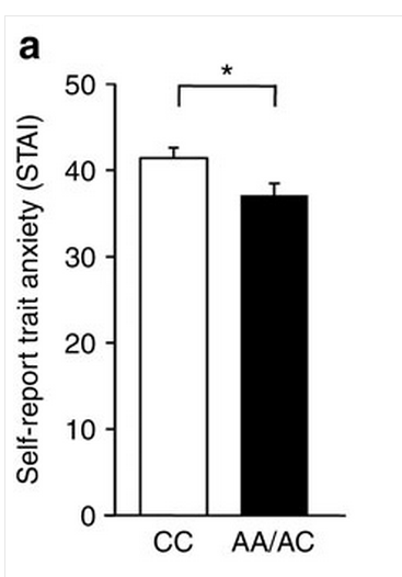
There’s good biological research behind this story, on how the gene works in both mice and people, but the impact is being oversold. The human data on anxiety in the paper look like

Combining this small difference with the claim that 20% of people  in the US carry the variant, it would explain about 1% of the population variation in the anxiety questionnaire score. Probably less of the variation in having/not having clinically diagnosable anxiety.

The story continues

“Those who do [have this mutation] may also be less likely to become addicted to marijuana and, possibly, other drugs – presumably because they don’t need the calming effects that marijuana provides.”

The New York Times version mentioned a study of marijuana dependence, which found people with the low-anxiety mutation were less likely to be dependent. However, for other drugs the opposite has been found:

Here, we report a naturally occurring single nucleotide polymorphism in the human FAAH gene, 385A, that is strongly associated with street drug use and problem drug/alcohol use.

People with the mutant, A, version of the gene, the low-anxiety variant, were more likely to have drug problems.  In fact, even the study that found (weak) evidence for lower rates of marijuana dependence found much stronger evidence of higher rates of sedative dependence.

Simple, binary, genetic explanations for complex human conditions are always tempting, but usually wrong.

• There will be SCIENCE at the Auckland Festival on Saturday: Dr Michelle ‘Nanogirl’ Dickinson blowing things up, Dr Siouxsie Wiles (and artists, and you) lighting things up, and panel discussions.

• ‘In the 17th century, another genre of paintings emerged, showing public administrators holding their books open for all to see. More than 100 of these paintings were produced between 1600 and 1800. Transparency became a cultural ideal worthy of art.’ Jacob Soll writing in the Boston Globe about the financial data revolution of the 16th century.

• “The next big milestone for the project is to get a judge to rule in favor of a tenant based on Heat Seek data. That would set a precedent that the courts see these devices as reliable and unbiased evidence.” New York, like many US cities, has temperature standards for apartments where the landlord controls the heating system. Heat Seek wants to provide independent data using internet-connected thermometers.

• Does the popularity of party leaders affect voting? In the UK it seems the answer is “sometimes, a bit”.  (via Alex Harrowell)

There are probably some StatChat readers who don’t read the NZ Herald, so I’ll point out that I have a post on the data blog about election donations.

A lot of statistical reporting focuses on means, or other summaries of where a distribution lies. Often, though, variation is important.  Vox.com has a story about variation in costs of lab tests at California hospitals, based on a paper in BMJ Open. Vox says

The charge for a lipid panel ranged from $10 to $10,169. Hospital prices for a basic metabolic panel (which doctors use to measure the body’s metabolism) were $35 at one facility — and $7,303 at another

These are basically standard lab tests, so there’s no sane reason for this sort of huge variation. You’d expect some variation with volume of tests and with location, but nothing like what is seen.

What’s not clear is how much this is really just variation in how costs are attributed. A hospital needs a blood lab, which has a lot of fixed costs. Somehow these costs have to be spread over individual tests, but there’s no unique way to do this.  It would be interesting to know if the labs with high charges for one test tend to have high charges for others, but the research paper doesn’t look at relationships between costs.

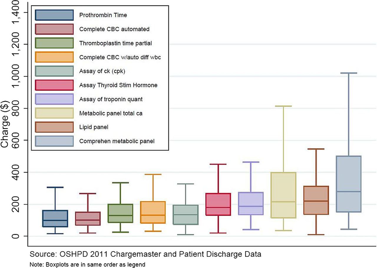
The Vox story also illustrates a point about reporting, with this graph

If you look carefully, there’s something strange about the graph. The brown box second from the right is ‘lipid panel’, and it goes up to a bit short of $600, not to $10169. Similarly, the ‘metabolic panel’, the right-most box, goes up to $1000 on the graph and $7303 in the story.

The graph is taken from the research paper. In the research paper it had a caption explaining that the ‘whiskers’ in the box plot go to the 5th and 95th percentiles (a non-standard but reasonable choice). This caption fell off on the way to Vox.com, and no-one seems to have noticed.