Posts filed under General (3156)

Team Ratings for Round 1

The basic method is described on my Department home page.

Here are the team ratings prior to this week’s games, along with the ratings at the start of the season.

Predictions for Round 1

Here are the predictions for Round 1. The prediction is my estimated expected points difference with a positive margin being a win to the home team, and a negative margin a win to the away team.

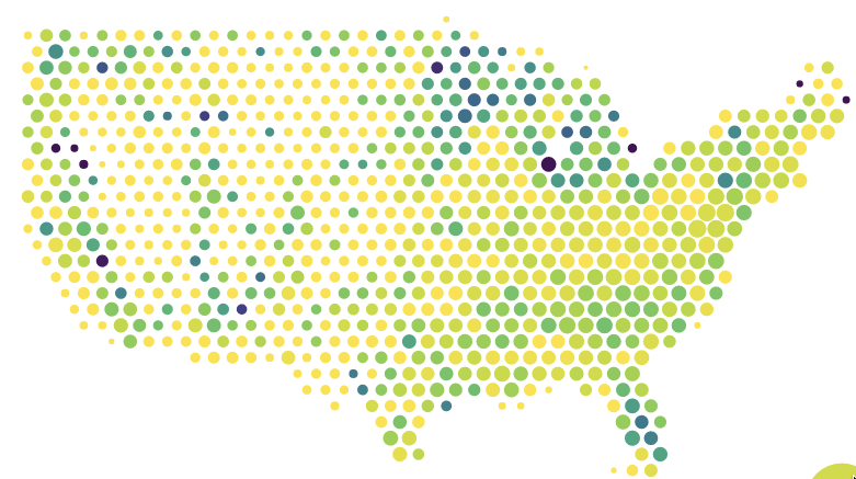
• “Places“:  Interactive maps of place name distribution in the US. For example “Lake” — with high density in the “Land of Lakes” but also in some less-expected places
• “Spreadsheets, the original analytics dashboard’, from Simply Statistics, about the origin of spreadsheets and what they were good for.

• Cats can see the ‘rotating snake’ optical illusion: video evidence from Rasmus Bååth

• As we’ve mentioned before, most people think teenagers have more risky behaviours now than in the Good Old Days. Most people are wrong. This time, from Vox.

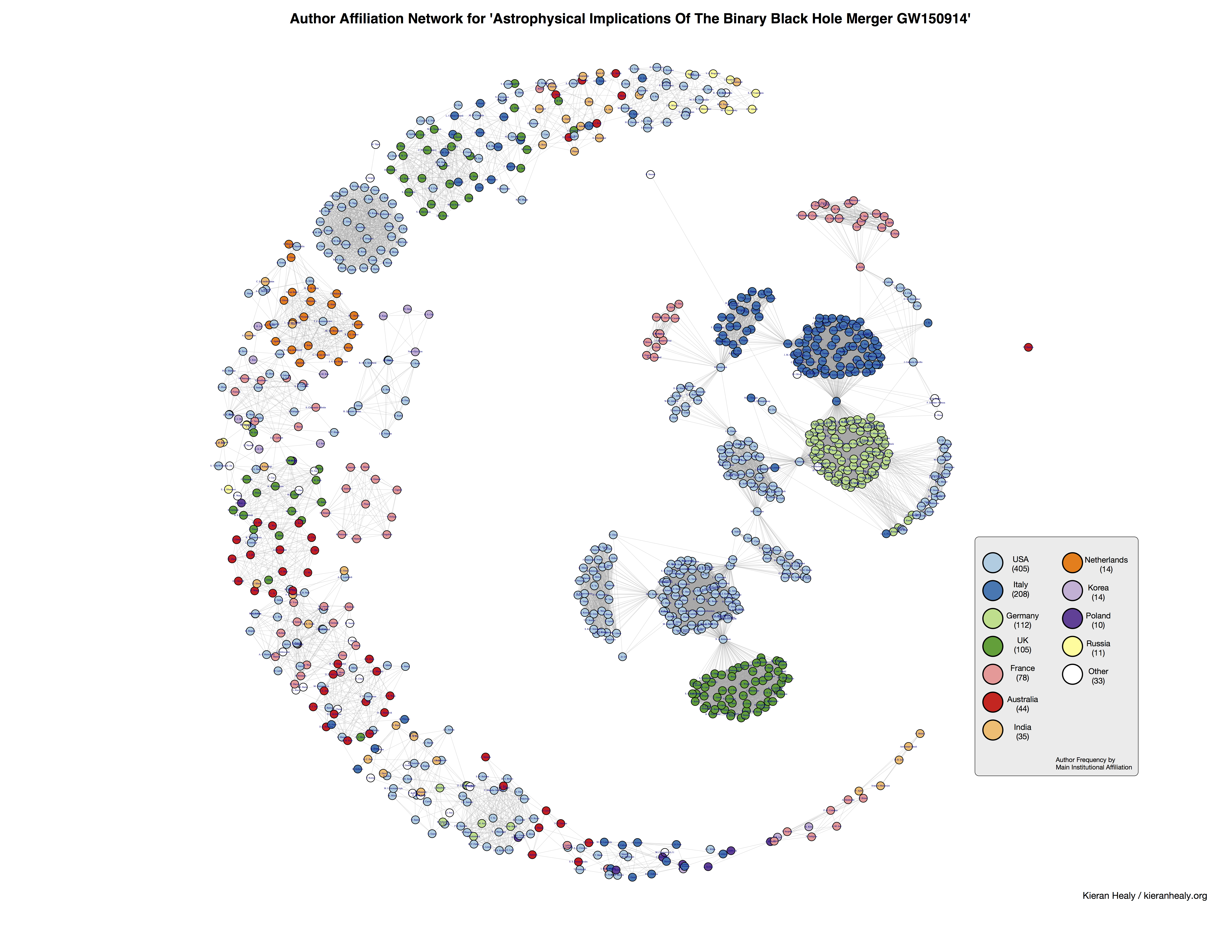
• From Kieran Healy, the network of shared institutional affiliations for the 1000+ authors of the LIGO gravitational waves paper (click to embiggen). That is, many scientists have some sort of connection with more than one university; the graph shows how these link up the LIGO researchers.
  
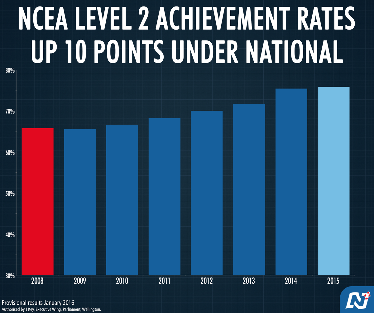
• Come on, major political parties. Barchart axes start at zero unless you want to look like Fox News. There are reasons for this. If you don’t want to start the axis at zero use some other sort of chart.
  

The Herald says “Police Minister Judith Collins has released figures to show crushing boy racers’ cars has worked“.  The data are more consistent with the political interpretation than is usual for claims about crashes, but not as strong as the Minister would like us to think.

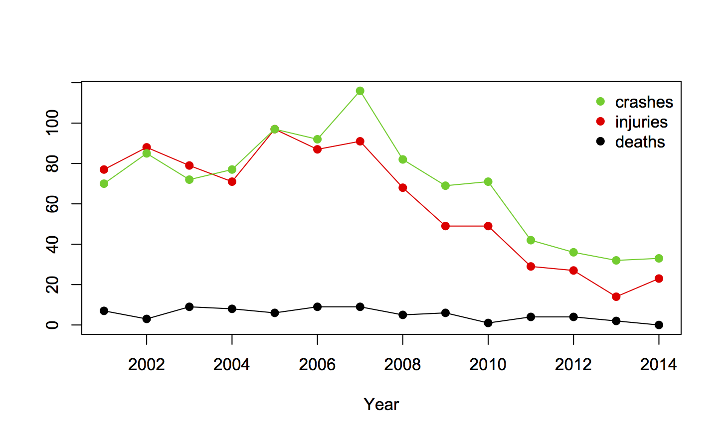
Here’s a graph of the data (supplied to the Herald by the Minister’s office), showing crashes, injuries, and deaths where the police reported ‘racing’ as a cause:

It’s fairly clear that something changed. Based purely on the graph you’d say the downwards trend started after 2007; 2009 isn’t unreasonable, but it fits the data a bit less well. This an example of a graph being much more useful than a table.

The next thing to check is other crashes — the road toll has been down in recent years, so this could just have been a general improvement. It’s not; the evidence for a change is a little weaker when considering racing deaths or injuries as a proportion of all fatal or injury crashes, but it’s still there.

In principle there could have been changes in reporting, but it’s hard to see how a government crackdown would make police less likely to report ‘racing’ involvement in a crash.

Finally, there’s publication bias.  The reporter, Nicholas Jones, didn’t notice that Ms Collins was back and decide to pull figures on car crushing; the Minister decided to release the figures. She wouldn’t have done that if they didn’t look favourable. It’s hard to tell how much to discount the evidence for that, but a discount is needed.

Overall, the data are definitely consistent with a deterrent effect of car crushing, but the evidence isn’t all that strong — the best fit to the data suggests things changed earlier than 2009, and looking at the numbers was the Minister’s idea, not the reporter’s.

Updates:

• in addition to the useful comments, I’ve been pointed to Dog & Lemon where Clive Matthew-Wilson says there is reason to believe the ‘boy racer’ thing was already going away on its own.  If so, that would fit the trend starting earlier than the legislation.
• If you check the crash numbers against the Road Crash Statistics system they don’t match.  I think that’s because Table 26 of the Road Crash Statistics only includes crashes causing injury or death — that’s explicit in the 2012 spreadsheet, and I think it’s still true.

One of the early motivating applications for linear mixed models was agricultural field studies looking at animal breeding or plant breeding. These are statistical models that combine differences between groups of observations with correlations between similar observations in order to get better comparisons.

John Oliver’s “Last Week Tonight” argues that these models shouldn’t be used to evaluate teachers , because they have been useful in animal breeding (with suitable video footage of a bull mounting a cow).  It’s really annoying when someone bases a reasonable conclusion on totally bogus arguments.

As the American Statistical Association has said on value-added models for teaching (PDF), the basic idea makes some sense, but there are a lot of details you have to get right for the results to be useful. That doesn’t mean rejecting the whole idea of considering the different ways in which classes can be different, or giving up on averages over relevant groups. On the other hand, the mere fact that someone calls something a “value-added model” doesn’t mean it tells you some deep truth.

It would be a real sign of progress if we could discuss whether a model adequately captures educational difficulties due to deprivation and family advantage without automatically rejecting it because it also applies to cows, or without automatically accepting it because it has the words “value-added.”

But it probably wouldn’t be as funny.

2016, NZ Herald, “A new report claims the world is heading for a chocolate deficit” (increased demand, no increase in supply)

There’s not much detail in the story, and I’m not going to provide any more because the report costs £1,700.00 (+VAT if applicable) — so remember, anything you read about it is just marketing.  However, there are other useful forms of context.

2013: Daily Mirror, “Chocolate could run out by 2020”

2012: NZ Herald, “Shortage will be costly for chocaholics”

2010: Discovery Channel, “Chocolate Supply Threatened by Cocoa Crisis”

2010: Independent, “Chocolate will be worth its weight in gold in 2020”

2008, CNN,”I think that in 20 years chocolate will be like caviar,”

2007:  MSN Money, “World chocolate shortage ahead”

2006: Financial Post, “Possible chocolate shortage ahead”

2002, Discover, “Endangered chocolate”

1998, New York Times, “Chocoholics take note: beloved bean in peril” (predicting a shortfall in “as little as 5-10 years”)

It could be that, like bananas, chocolate really always is in peril, or it could be that falling global inequality will make it much more expensive, or it could be that it’s just a good story.

From Stuff

“According to a new study titled, Music Makes it Home, couples who listen to music together saw a huge spike in their sex lives.”

This is a genuine experimental study, but it’s for marketing. Neither the design nor the reporting are done they way they would be if the aim was to find things out.

In addition to a survey of 30,000 people, which just tells you about opinions, Stuff says Sonos did an experiment with 30 families:

Each family was given a Sonos sound system and Apple Music subscription and monitored for two weeks. In the first week, families were supposed to go about their lives as usual. But in the second week, they were to listen to the music.

Sonos says

The first week,participants were instructed not to listen to music out loud. The second week,participants were encouraged to listen to music out loud as much as they wanted.

That’s a big difference.

The reporting, both from Sonos and from Stuff, mixes results from the 30,000-person survey in with the experiment results.  For example, the headline statistic in the Stuff story, 67% more sex, is from the survey, even though the phrasing “saw a huge spike in their sex lives” makes it sound like a change seen in the experiment. The experimental study found 37% more ‘active time in the bedroom’.

Overall, the differences seen in the experimental study still look pretty impressive, but there are two further points to consider.  First, the participants knew exactly what was going on and why, and had been given lots of expensive electronics.  It’s not unreasonable to think this might bias the results.

Second, we don’t have complete results, just the summaries that Sonos has provided — it wouldn’t be surprising if they had highlighted the best bits. In fact, the neuroscientist involved with the study admits in the story that negative results probably wouldn’t have been published.

Q: Did you see there’s a new, 100% accurate cancer test?

A: No.

Q: It only uses a bit of saliva, and it can be done at home?

A: No.

Q: No?

A: Remember what I’ve said about ‘too good to be true’?

Q: So how accurate is it?

A: ‘It’ doesn’t really exist?

Q: But it “will enter full clinical trials with lung cancer patients later this year.”

A: That’s not a test for cancer. The phrase “lung cancer patients” is a hint.

Q: So what is it a test for?

A: It’s a test for whether a particular drug will work in a patient’s lung cancer

Q: Oh. That’s useful, isn’t it?

A: Definitely

Q: And that’s 100% accurate?

A: <tilts head, raises eyebrows>

Q: Too good to be true?

A: The test is very good at getting the same results that you would get from analysing a surgical specimen. Genetically it’s about 95% accurate in a small set of data reported in January. In clinical trials, 50% of people with the right tumour genetics responded to the drug. So you could say the test is 95% accurate or 50% accurate.

Q: That still sounds pretty good, doesn’t it?

A: Yes, if the trial this year gets results like the preliminary data it would be very impressive.

Q: And he does this with just a saliva sample?

A: Yes, it turns out that a little bit of tumour DNA ends up pretty much anywhere you look, and modern genetic technology only needs a few molecules.

Q: Could this technology be used for detecting cancer, too?

A: In principle, but we’d need to know it was accurate. At the moment, according to the abstract for the talk that prompted the story, they might be able to  detect 80% of oral cancer. And they don’t seem to know how often a cell with one of the mutations might turn up in someone who wouldn’t go on to get cancer. Since oral cancer is rare, the test would need to be extremely accurate and inexpensive to be worth using in healthy people.

Q: What about other more common cancers?

A: In principle, maybe, but most cancers are rare when you get down to the level of specific genetic mutations.  It’s conceivable, but it’s not happening in the two-year time frame that the story gives.

As I said in August

“How would you even study that?” is an excellent question to ask when you see a surprising statistic in the media. Often the answer is “they didn’t,” but sometimes you get to find out about some really clever research technique.

There are stories around, such as the one in Stuff, about modern disease due to Neanderthal genes (press release).

The first-ever study directly comparing Neanderthal DNA to the human genome confirmed a wide range of health-related associations — from the psychiatric to the podiatric — that link modern humans to our broad-browed relatives.

It’s basically true, although as with most genetic studies the genetic effects are really, really small. There’s a genetic variant that doubles your risk of nicotine dependence, but only 1% of Europeans have it. The researchers estimate that Neanderthal genetic variants explain about 1% of depression and less than half  a percent of cardiovascular disease. But that’s not zero, and it wasn’t so long ago that the idea of interbreeding was thought very unlikely.

Since hardly any Neanderthals have had their genome sequenced, how was this done? There are two parts to it: a big data part and a clever genetics part.

The clever genetics part (paper) uses the fact that Neanderthals and modern humans, since their ancestors had been separated for a long time (350,000 years), had lots of little, irrelevant differences in DNA accumulated as mutations– like a barcode sequence.  Given a long enough snippet of genome, we can match it up either to the modern human barcode or the Neanderthal barcode. Neanderthals are recent enough (50,000 years is maybe 2500 generations) that many of the snippets of Neanderthal genome we inherit are long enough to match up the barcodes reliably.  The researchers looked at genome sequences from the 1000 Genomes Project, and found genetic variants existing today that are part of genome snippets which appear Neanderthal.  These genetic variants are what they looked at.

The Big Data is a collection of medical records at nine major hospitals in the US, together with DNA samples. This nothing like a random sample, and the disease data are from ICD9 diagnostic codes rather than detailed medical record review, but quantity helps.

Using the DNA samples, they can see which people have each of the  Neanderthal-looking genetic variants, and what diseases these people have — and find the very small differences.

This isn’t really medical research. The lead researcher quoted in the news is an evolutionary geneticist, and the real story is genetics: even though the Neanderthals vanished 50,000 years ago, we can still see enough of their genome to learn new things about how they were different from us.

The LIGO gravitational wave detector is an immensely complex endeavour, a system capable of detecting minute gravitational waves, and of not detecting everything else.

To this end, the researchers relied on every science from astronomy to, well, perhaps not zymurgy, but at least statistics. If you want to know “did we just hear two black holes collide?” it helps to know what it will sound like when two black holes collide right at the very limit of audibility, and how likely you are to hear noises like that just from motorbikes, earthquakes, and Superbowl crowds.  That is, you want a probability model for the background noise and a probability model for the sound of colliding black holes, so you can compute the likelihood ratio between them — how much evidence is in this signal.

One of the originators of some of the methods used by LIGO is Renate Meyer, an Associate Professor in the Stats department. Here’s her comments to the Science Media Centre, and a post on the department website

NPR’s Planet Money ran an interesting podcast in mid-January of this year. I recommend you take the time to listen to it.

The show discussed the idea that there are problems in the way that we do science — in this case that our continual reliance on hypothesis testing (or statistical significance) is leading to many scientifically spurious results. As a Bayesian, that comes as no surprise. One section of the show, however, piqued my pedagogical curiosity:

STEVE LINDSAY: OK. Let’s start now. We test 20 people and say, well, it’s not quite significant, but it’s looking promising. Let’s test another 12 people. And the notion was, of course, you’re just moving towards truth. You test more people. You’re moving towards truth. But in fact – and I just didn’t really understand this properly – if you do that, you increase the likelihood that you will get a, quote, “significant effect” by chance alone.

KESTENBAUM: There are lots of ways you can trick yourself like this, just subtle ways you change the rules in the middle of an experiment.

You can think about situations like this in terms of coin tossing. If we conduct a single experiment where there are only two possible outcomes, let us say “success” and “failure”, and if there is genuinely nothing affecting the outcomes, then any “success” we observe will be due to random chance alone. If we have a hypothetical fair coin — I say hypothetical because physical processes can make coin tossing anything but fair — we say the probability of a head coming up on a coin toss is equal to the probability of a tail coming up and therefore must be 1/2 = 0.5. The podcast describes the following experiment:

KESTENBAUM: In one experiment, he says, people were told to stare at this computer screen, and they were told that an image was going to appear on either the right site or the left side. And they were asked to guess which side. Like, look into the future. Which side do you think the image is going to appear on?

If we do not believe in the ability of people to predict the future, then we think the experimental subjects should have an equal chance of getting the right answer or the wrong answer.

The binomial distribution allows us to answer questions about multiple trials. For example, “If I toss the coin 10 times, then what is the probability I get heads more than seven times?”, or, “If the subject does the prognostication experiment described 50 times (and has no prognostic ability), what is the chance she gets the right answer more than 30 times?”

When we teach students about the binomial distribution we tell them that the number of trials (coin tosses) must be fixed before the experiment is conducted, otherwise the theory does not apply. However, if you take the example from Steve Lindsay, “..I did 20 experiments, how about I add 12 more,” then it can be hard to see what is wrong in doing so. I think the counterintuitive nature of this relates to general misunderstanding of conditional probability. When we encounter a problem like this, our response is “Well I can’t see the difference between 10 out of 20, versus 16 out of 32.” What we are missing here is that the results of the first 20 experiments are already known. That is, there is no longer any probability attached to the outcomes of these experiments. What we need to calculate is the probability of a certain number of successes, say x given that we have already observed y successes.

Let us take the numbers given by Professor Lindsay of 20 experiments followed a further 12. Further to this we are going to describe “almost significant” in 20 experiments as 12, 13, or 14 successes, and “significant” as 23 or more successes out of 32. I have chosen these numbers because (if we believe in hypothesis testing) we would observe 15 or more “heads” out of 20 tosses of a fair coin fewer than 21 times in 1,000 (on average). That is, observing 15 or more heads in 20 coin tosses is fairly unlikely if the coin is fair. Similarly, we would observe 23 or more heads out of 32 coin tosses about 10 times in 1,000 (on average).

So if we have 12 successes in the first 20 experiments, we need another 11 or 12 successes in the second set of experiments to reach or exceed our threshold of 23. This is fairly unlikely. If successes happen by random chance alone, then we will get 11 or 12 with probability 0.0032 (about 3 times in 1,000). If we have 13 successes in the first 20 experiments, then we need 10 or more successes in our second set to reach or exceed our threshold. This will happen by random chance alone with probability 0.019 (about 19 times in 1,000). Although it is an additively huge difference, 0.01 vs 0.019, the probability of exceeding our threshold has almost doubled. And it gets worse. If we had 14 successes, then the probability “jumps” to 0.073 — over seven times higher. It is tempting to think that this occurs because the second set of trials is smaller than the first. However, the phenomenon exists then as well.

The issue exists because the probability distribution for all of the results of experiments considered together is not the same as the probability distribution for results of the second set of experiments given we know the results of the first set of experiment. You might think about this as being like a horse race where you are allowed to make your bet after the horses have reached the half way mark — you already have some information (which might be totally spurious) but most people will bet differently, using the information they have, than they would at the start of the race.